|
|
|
We have designed a PID control loop simulator using Matlab and Simulink. Below is the PID control loop graphically designed using Simulink (Matlab and Simulink are excellent software design tools developed by The MathWorks Inc). The PID controller we have implemented is of type C. For more info about different types of PID controller please visit http://bestune.50megs.com/type_ABC.htm.
The PID controller contains a built in digital filter. It receives 8 inputs:
x(1): Filtered PV, which will be further filtered in the built in digital
filter.
x(2): Setpoint.
x(3): The proportional gain Kp.
x(4): The integral gain Ki.
x(5): The derivative gain Kd.
x(6): Time.
x(7): If it is 1, then use PID control action, otherwise use manual CO value.
x(8): Manual CO value.
The PID controller plus a built in digital filter is designed as a Matlab function "pid1.m", as shown below.
function u=pid(x)
global Tpid
Tf t0 t1 tf k
global sp
ek uk uk_1 yk yk_1 vk vk_1
% Digital filter and PID control
% Designed by BESTune Comp.
% WWW: http://bestune.50megs.com
% Copyright 1998-2002
t=x(6); % Read time
if t==0
k=0;
Tpid=1; % PID loop
update time
t0=0;
t1=0;
uk=x(8); % Initial CO value
yk=x(1); %
Initial PV value
sp=x(2); %
Initial setpoint
ek=sp-yk;
Tf=0.1; % Filter
time constant
tf=200; % Simulation stop time
else %
Filtering yk
T0=t-t0;
yk=yk*Tf/(Tf+T0)+x(1)*T0/(Tf+T0);
t0=t;
end
% End of the filter.
% The filtered yk will be used to
% (1)calculate PID control and
% (2)tune the PID controller
% Beginning of the PID controller
if t-t1>=Tpid
| x(2)~=sp %Every Tpid sec calculate the new CO value
sp=x(2);
T=t-t1;
if T>0.0001 %Avoid division by T=0
if x(7)==1 & k>=3 % Then use PID
control
Kp=x(3);
Ki=x(4);
Kd=x(5);
ek=sp-yk;
vk=(yk-yk_1)/T;
ak=(vk-vk_1)/T;
Du=(Ki*ek-Kp*vk-Kd*ak)*T;
uk=uk_1+Du*T;
else
if k>=1 vk=(yk-yk_1)/T; end
if k>=2 ak=(vk-vk_1)/T; end
uk=x(8); % Use manual uk value x(8)
k=k+1;
end
end
if uk>5 uk=5;end % uk must be <= upper limit
if uk<-5
uk=-5;end % uk must be >= lower limit
% Show the control results and update t1, yk_1, vk_1, uk_1
fprintf('time=%5.2f setpoint=%5.2f pv=%5.2f co=%5.2f\n',t,x(2),yk,uk)
t1=t;yk_1=yk;vk_1=vk;uk_1=uk;
end
% End of the PID controller
u=uk;
The filter part is scaned at a very high
frequency (i.e., every T0 seconds the filter will be executed once and T0 is
very small). The PID controller is executed every Tpid=1 seconds.
Please note that the filter design and PID controller design are separated. When you tune this PID controller, the filter should be considered as a part of the process. So strictly speaking each time when you make changes to the filter, you should re-tune your PID parameters.
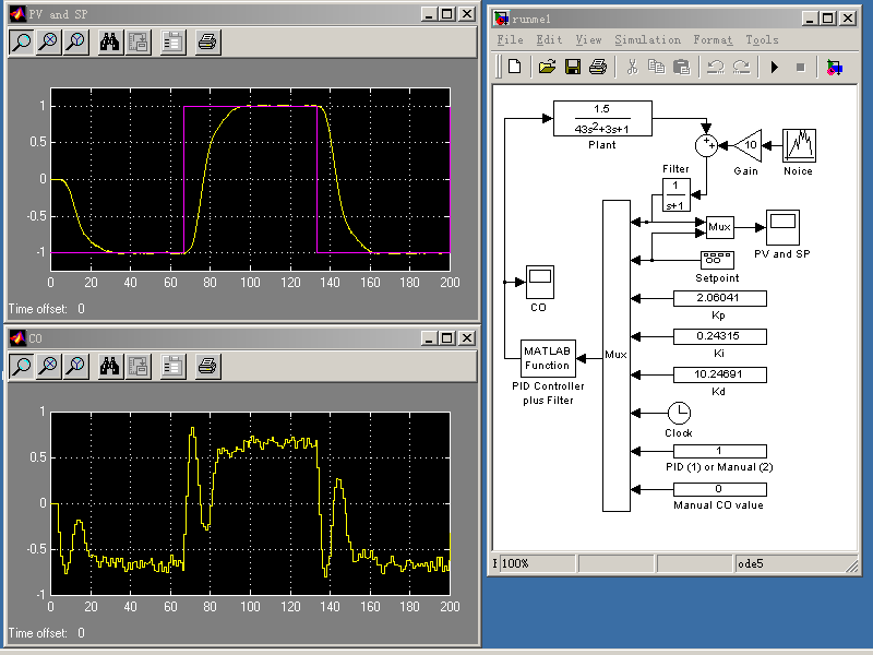
The above simulator uses two files: runme1.mdl and pid1.m, which can be download by clicking on this link.
There are many PID controller auto-tuning tools on the market. How to rate their quality? One thing you can do is to use the following "pid2.m" to replace the above "pid1.m". The major advantage of this function is that it automatically generates a data file "co_pv.txt" when the simulation finishes. The sampling period used to sample the CO and PV data is Ts=1 second. You can provide this "co_pv.txt" file to people with PID controller auto-tuning tools and ask them to return you the values of Kp, Ki, and Kd. You also need to tell them the sampling period Ts and the process dead-time if they so ask. You can then test the performance of the retuned PID loop and hence rate the quality of their PID controller auto-tuning tools. If you want to test the quality of BESTune, you can send your co_pv.txt file to bestune@gmail.com and we will return the tuning results to you. Before doing this, you may want to change the structure of your plant. Remember, you should keep the structure of your plant (e.g., the transfer function of the plant) secret, because in practical situations all we can get are measurements of CO and PV, not the exact model of the plant. However, if the transfer function of the process is known, we can get almost perfect PID controllers. Take a look at http://bestune.50megs.com/more.htm for more about this.
In the above case the parameter Ki=0.24315 may be too small to implement on some PID controllers. Please note that the integral term is essential and we cannot set Ki=0. One solution to this problem is scaling. The following "pid2.m" magnifies the three tuning constants by g=10 times without affecting the performance of the PID controller at all.
function u=pid(x)
global Tpid
Ts Tf t0 t1 t2 tf k
global sp
ek uk uk_1 yk yk_1 vk vk_1 co_pv
% Digital filter and PID control
% Designed by BESTune Comp.
% WWW: http://bestune.50megs.com
% Copyright 1998-2002
t=x(6); % Read time
g=10; % scale gain
x(1)=x(1)/g; %
scale PV
x(2)=x(2)/g; %
scale SP
if t==0
k=0;
Tpid=1; % PID loop
update time
Ts=1; %
Sampling period for data CO and PV
t0=0;
t1=0;
t2=0;
co_pv=[];
uk=x(8); % Initial CO value
yk=x(1); %
Initial PV value
sp=x(2); %
Initial Setpoint
ek=sp-yk;
Tf=0.1; % Filter
time constant
tf=200; % Simulation stop time
else %
Filtering yk
T0=t-t0;
yk=yk*Tf/(Tf+T0)+x(1)*T0/(Tf+T0);
t0=t;
end
% End of the filter.
% The filtered yk will be used to
% (1)calculate PID control and
% (2)tune the PID controller
% Beginning of the PID controller
if t-t1>=Tpid
| x(2)~=sp %Every Tpid sec calculate the new CO value
sp=x(2);
T=t-t1;
if T>0.0001 %Avoid division by T=0
if x(7)==1 & k>=3 % Then use PID
control
Kp=x(3);
Ki=x(4);
Kd=x(5);
ek=sp-yk;
vk=(yk-yk_1)/T;
ak=(vk-vk_1)/T;
Du=(Ki*ek-Kp*vk-Kd*ak)*T;
uk=uk_1+Du*T;
else
if k>=1 vk=(yk-yk_1)/T; end
if k>=2 ak=(vk-vk_1)/T; end
uk=x(8); % Use manual uk value x(8)
k=k+1;
end
end
if uk>5
uk=5;end % uk must be <= upper limit
if uk<-5 uk=-5;end % uk must be >= lower limit
if t+Tpid>=tf % Before simulation ends, save co and pv
save co_pv.txt co_pv -ascii
end
% Show the control results and update t1, yk_1, vk_1, uk_1
fprintf('time=%5.2f setpoint=%5.2f pv=%5.2f co=%5.2f\n',t,x(2),yk,uk)
t1=t;yk_1=yk;vk_1=vk;uk_1=uk;
end
% End of the PID controller
% Sample CO and PV data every Ts seconds
if t-t2>=Ts
co_pv=[co_pv;uk yk]; %Every Ts sec sample co and pv once
t2=t; % Update t2
end
u=uk;
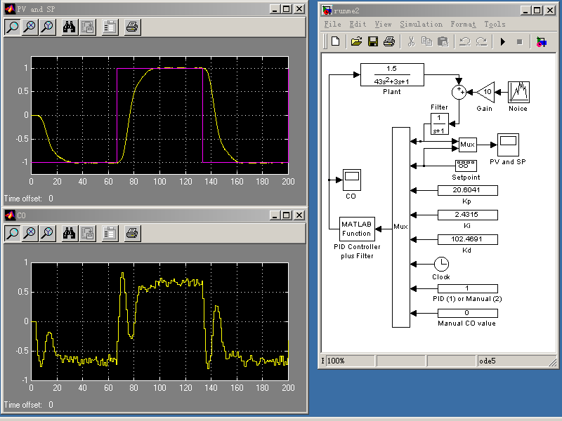
The above simulation uses two files: runme2.mdl and pid2.m, which can be download by clicking on this link.
This second simulator will give the following simulation result. Please note that all the three tuning constants Kp, Ki, and Kd are amplified by g=10 times, and the performance of the PID controller is exactly the same as the above PID controller.